Wow! Transformers Learn Factored Representations
July 11, 2026
While today’s transformer-based language models are good at understanding and generating text, the way they work on the inside remains… mysterious. Recently, Shai et al. published a paper in ICML this year titled Transformers learn factored representations that aims to shed light on this subject.
The authors asked whether transformer models, on their own, decompose their understanding of the world into discrete, independent factors or components. Here, they took inspiration from human beings, who naturally parse sensory input into discrete objects and concepts.
Humans take this stream of raw data, and decompose it into discrete objects—chairs, coffee mugs, other agents—in order to understand the world. Do transformers also learn to factor their world into parts? How can they from a mere stream of tokens, and why would they?
Shai et al., §1
They ask if these models exhibit an inherent “inductive bias” towards learning factored representations (that is, do they break down complex information into separate, orthogonal subspaces rather than representing everything together in a tangled, high-dimensional space)? If transformers trained on next-token prediction learn to factor their internal model of the world into constituent parts (especially if not explicitly made to do so) this would represent a trade off between “predictive accuracy” with “representational efficiency” and transformers preferring the latter approach. And it turns out they do!
Transformers pretrained via next token prediction learn to factor their world into parts, representing these factors in orthogonal subspaces of the residual stream. We formalize two representational hypotheses:
(1) a representation in the product space of all factors, whose dimension grows exponentially with the number of parts, or
(2) a factored representation in orthogonal subspaces, whose dimension grows linearly.
Shai et al., Abstract
How did they discover this?
Mathematical Foundations
The authors’ framework centers on Generalized Hidden Markov Models (GHMMs), which model how token sequences are generated by underlying latent processes.
To explain GHMMs, imagine a street corner with five vendors standing in a row prepared to sell you fruits. But you don’t get to pick the fruits. The vendor sells you whatever fruit they feel like according to their mood.
Let’s say for three of the five vendors, they have three moods (akin to what the paper calls mess3 factor). There’s an apple mood (🍎mood), banana mood (🍌mood), and pear mood (🍐mood). Now if a vendor is of a particular mood there’s an 80% chance she sells you the fruit corresponding to that mood, and a 20% chance she sells you some other fruit. Concretely:
-
🍎mood: 80% 🍎, 10% 🍌, 10% 🍐
-
🍌mood: 10% 🍎, 80% 🍌, 10% 🍐
-
🍐mood: 10% 🍎, 10% 🍌, 80% 🍐
So if you get an apple, what mood is the vendor in? Well. That’s where EVERYONE’S FAVORITE THEOREM, Bayes’ theorem, comes in:
$$P(A|B) = \frac{P(B|A) P(A)}{P(B)}$$What is the probability the vendor is in an apple kinda mood given that she gave us an apple.
$$ \begin{aligned} P(\text{mood} \mid \text{fruit}) &= \frac{P(\text{fruit} \mid \text{mood}) \cdot P(\text{mood})}{P(\text{fruit})} \\[6pt] P(🍎\text{mood} \mid 🍎) &= \frac{P(🍎 \mid 🍎\text{mood}) \cdot P(🍎\text{mood})}{P(🍎)} \\[6pt] &= \frac{0.8 \cdot \frac{1}{3}}{\frac{1}{3}} = 0.8 \end{aligned} $$Great, so that particular vendor has an 80% chance of being in an apple mood. Now, after selling us the fruit, the vendor’s mood changes and this is also determined by probability:
-
In 🍎 mood: 80% stay 🍎, 10% switch to 🍌, 10% switch to 🍐
-
In 🍌 mood: 10% switch to 🍎, 80% stay 🍌, 10% switch to 🍐
-
In 🍐 mood: 10% switch to 🍎, 10% switch to 🍌, 80% stay 🍐
So a run might look something like:
mood: 🍎 🍎 🍎 🍌 🍌 🍌 🍐 🍐 🍐 🍐 🍐 🍎 🍎 🍎
shout: 🍎 🍎 🍌 🍌 🍎 🍌 🍐 🍐 🍎 🍐 🍎 🍎 🍎 🍎
The other two vendors pick their fruits according to what Shai et al. call the “Bloch Walk.” Here, these vendors have four fruits on their menu (🍇, 🍋, 🍈, 🥝) and they select fruits by, instead of having discrete moods, their mood is the location of a dot somewhere on a flat 2D disk sitting inside a ball1.
Where the dot is sets the odds on the four fruits. Each of the four fruits has an anchor point on the disk. The closer the dot is to a fruit’s anchor, the more likely that fruit. The odds slide smoothly as the dot moves around, and the four always add up to 1. After each sale the dot drifts (“walks”) to a new spot in the disk.
Here, a run might look something like
mood: (0.5, 0.1) (0.42, 0.18) (0.31, 0.22) (0.15, 0.28) (-0.05, 0.31)
shout: 🍋 🍇 🍇 🍈 🍈
Where the ball traces a path on the qubit like
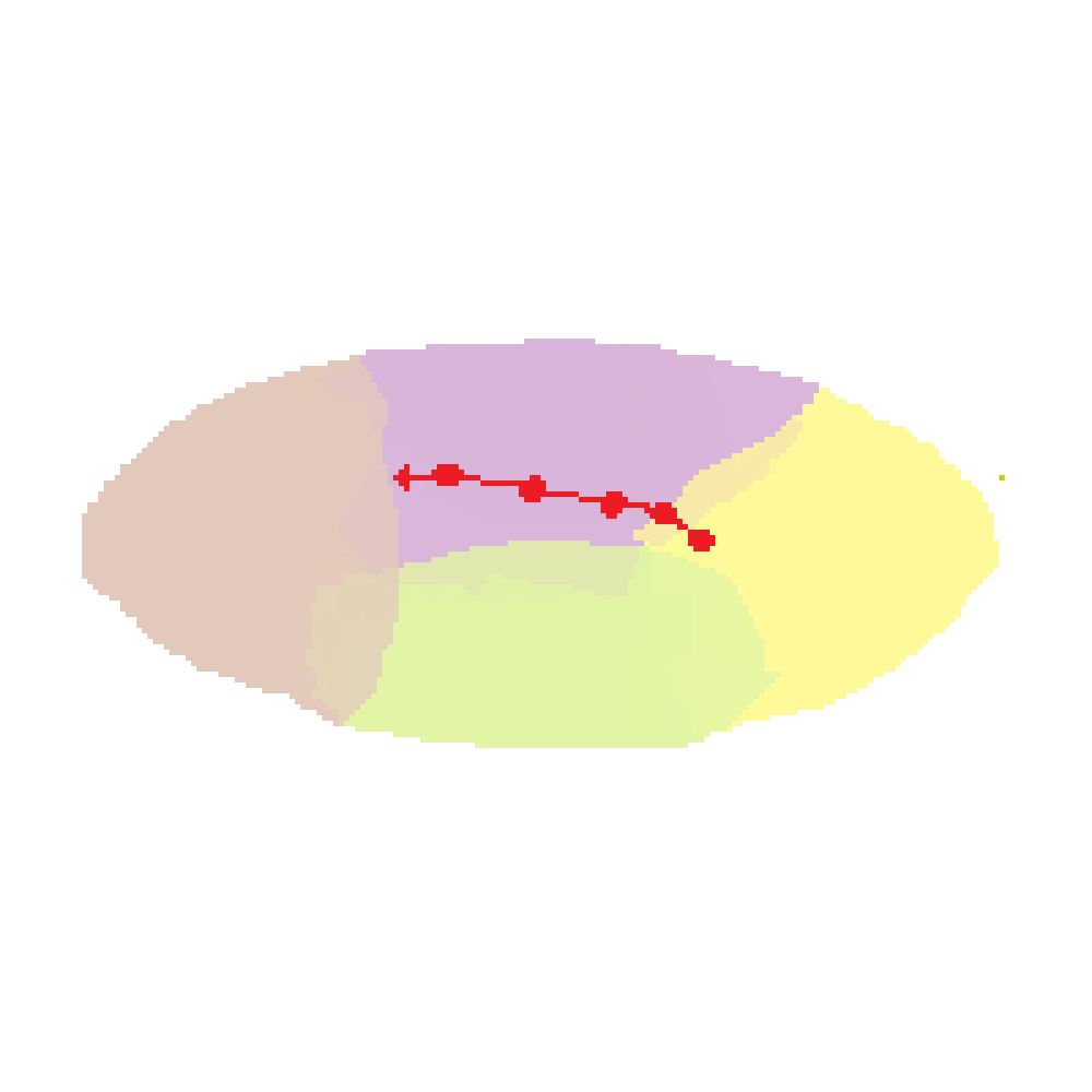
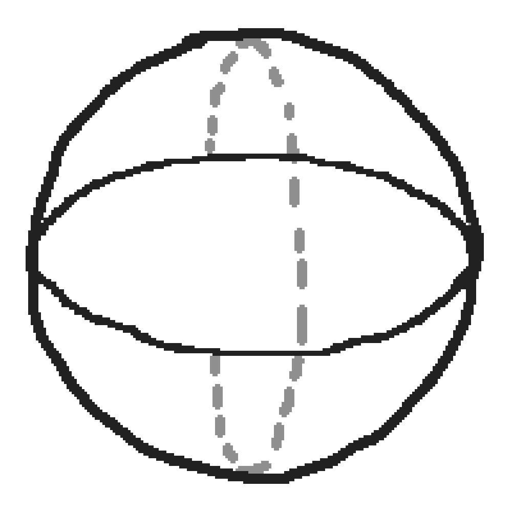 The dot’s path on the Bloch ball as the vendor’s mood drifts across the four fruits.
Now all five vendors are selling you their fruit at the same time, what’s more is that these fruits are blended into a smoothie and you don’t get to see who sells you what. (You don’t really have a great sense of taste.) You can’t really tell how many of what particular fruits are in a smoothie but you can tell if you’ve had a smoothie before. Let’s represent the smoothies as a tuple:
smoothie 326 = (🍎, 🍎, 🍌, 🍇, 🍈)smoothie 073 = (🍐, 🍌, 🍎, 🍈, 🥝)smoothie 217 = (🍌, 🍎, 🍌, 🍈, 🍇)...// and so on
Having all five street vendors make a smoothie at once is akin to a “composite generator” its “transition operator” is built from the five individual vendors.
$$T^{(x)} = \bigotimes_{n=1}^{5} T_n^{(x_n)}$$
Such a multi-partite generator has latent space $\mathcal{S}=\bigotimes_{n=1}^{N}\mathcal{S}_n$, the tensor product of $N$ constituent latent spaces.
Shai et al., §2.3
A transition operator is the rule for updating your guess about a vendor’s mood after they hand you a fruit. That guess is a set of probabilities over the moods that gets nudged by each fruit. The tensor product ($\bigotimes$) tracks every combination of the five moods at once, which is why the sizes multiply instead of add.
That is to say, $3 \times 3 \times 3 \times 4 \times 4 = 432$ different possible smoothies! Each of the 432 smoothie-tuples gets an arbitrary integer from 0 to 431. Also note that adjacent numbers mean nothing. Smoothie 47 might be (🍌, 🍌, 🍌, 🍈, 🥝) whereas smoothie 48 might be (🍐, 🍐, 🍐, 🍎, 🍎). Recall that we cannot taste which particular fruits went into a smoothie. Now, each smoothie implies something about the mood of each of the vendors.
Predicting the Next Smoothie
To predict the next tuple, an ideal predictor would understand, at every step, each vendor’s current belief about its mood. The paper calls this the predictive vector $\eta^{(x_{1:\ell})}$.
[W]hat does the model need to know to predict optimally? Only the information the past reveals about the future [...] We call the vector encoding this information the predictive vector [...] Two contexts with identical predictive vectors make identical predictions about all future tokens.
Shai et al., §2.2
We build this from a prior $\eta^{(\varnothing)}$, applying one transition operator per fruit and renormalizing so the numbers sum to 1:
$$\eta^{(x_{1:t})} = \frac{\eta^{(\varnothing)} T^{(x_1)} \cdots T^{(x_t)}}{\eta^{(\varnothing)} T^{(x_1)} \cdots T^{(x_t)} \mathbf{1}}$$For one three-mood vendor, that belief is three numbers (how much you’d bet on 🍎, 🍌, 🍐) summing to 1.
Every such trio is a point in a triangle where being at a corner means total certainty about one mood, the dead center is a three-way coin flip, an edge means one mood is ruled out. This is called a “2-simplex” because once we know two of the numbers, we know where the third has to be.
Naively, the joint belief lives in the product space of every combination of the five vendors’ beliefs. Each vendor’s belief is a 3-number vector2, so the joint stacks to $\prod_n d_n = 3^5 = 243$ dimensions (or $242$ after each belief is normalized).
Direct Sum
Since the vendors are independent (that is nobody’s mood depends on anyone else’s) the joint belief factors. It’s a product state, $\eta = \bigotimes_n \eta_n$ where the giant joint table is the five individual beliefs multiplied out into every combination.
For $N$ factors with latent dimensions $d_1,\ldots,d_N$, [the joint] requires $(\prod_n d_n)-1$ dimensions [while the] factored requires only $\sum_n(d_n-1)$ dimensions—exponentially fewer.
Shai et al., §2.4
$N$ is the number of factors (here, our five vendors) and $d_n$ is the “latent dimension” of factor $n$, i.e. how many numbers it takes to write down that one vendor’s belief. $\prod_n d_n$ multiplies those sizes together (every combination of beliefs at once) while $\sum_n(d_n-1)$ just adds up each vendor’s degrees of freedom.
The authors prove that whenever the generator factors into independent parts, a lossless linear map into orthogonal subspaces exists.
The Factored World Hypothesis
Transformers have an inductive bias toward factored representations, organizing their activations into a direct sum of low-dimensional orthogonal subspaces even when higher-dimensional representations would be more faithful.
Shai et al., §2.5
Which means that
[A]ctivations should concentrate in $\sum_n(d_n-1)$ dimensions, not $(\prod_n d_n)-1$ [...] [and] these dimensions should organize into $N$ orthogonal subspaces, one per factor.
Shai et al., §2.6
Our residual stream is 120 numbers wide, which, while nowhere near enough to hold the naïve 242-dimension joint belief, is twelve times what the 10-dim factored one needs. (The joint belief is written as 243 numbers, but it’s always a product of the five vendor beliefs and therefore only ever moves on a 10-dim surface.) The model must compress. While it could smear those 10 dimensions across all 120 directions, it instead packs each vendor’s belief into its own roughly-orthogonal block ($V_1, \ldots, V_5 \subset \mathbb{R}^{120}$, with $V_n \perp V_m$) and leaves the rest of the stream empty.3
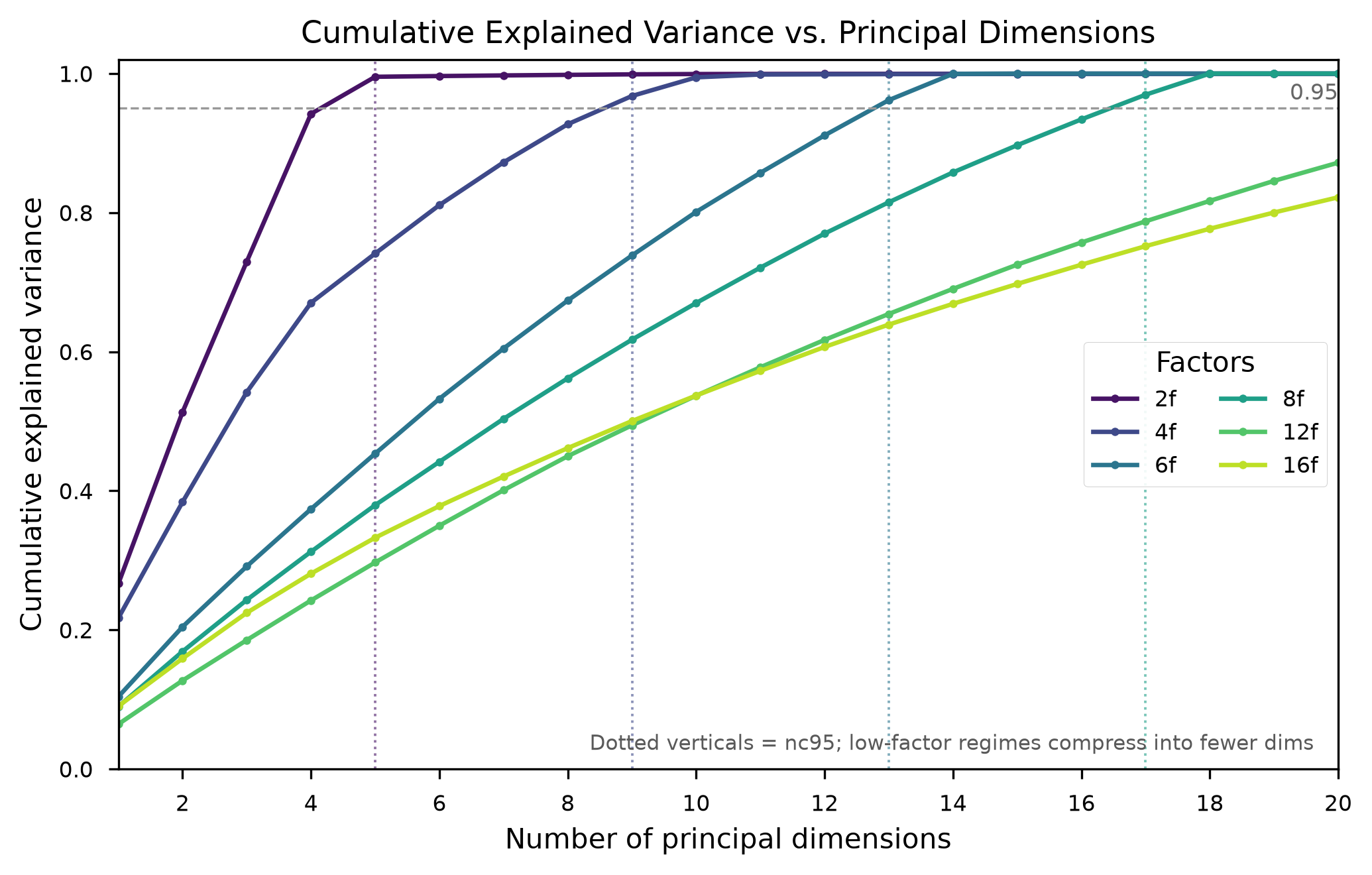 CEV per regime with variance concentrating in $\sum_n d_n$ dimensions
Orthogonal subspaces mean that changes to one subspace don’t interfere with others. If vendor 3’s block is perpendicular to the other four, you can read vendor 3’s belief off the stream without the others bleeding in, and change it by nudging the activation along that block without touching the rest.
This is the same premise behind steering (turn one concept up by adding a direction to the activations): a linear edit does one thing only if the concepts live in separate directions. So “are the factors orthogonal” is the difference between editing one attribute and secretly editing five.
The model seems to not only end up with a “factored” approach, it seems to actively routes through it first, even when factoring is a bad idea. The authors try this out by introducing noise:
With probability $1-\varepsilon$, the token is transmitted faithfully; with probability $\varepsilon$, it is replaced by a uniformly random token.
Shai et al., §4.3
Where $\varepsilon$ is a noise dial from 0 to 1. At $\varepsilon = 0$ every composite is honest, at $\varepsilon = 1$ the number is purely noise. Concretely:
$$T^{(z)} = \varepsilon\, T_{\text{int}} + (1-\varepsilon) \bigotimes_n T_n^{(z)}$$
Say two vendors, moods A/B, each emits the fruit of it’s mood % of the time, both 95% likely to be in A. You observe (🍎, 🍎) under $\varepsilon = 0.2$. Running Bayes over $\{AA, AB, BA, BB\} \times \{\text{faithful}, \text{noise}\}$, and marginalizing out the noise flag, yields $P(V_1 = A) = 0.885$ and $P(BB) = 0.027$ whereas a factored belief could only ever produce $P(BB) = P(B)^2 = 0.115^2 = 0.013$.
The noise, corrupting all emissions equally, affects all of them together, and yet:
The factored solution acts as a representational attractor. Models find it quickly, dwell there, and depart only under sustained gradient pressure [...] [T]ransformers first collapse to the [...] factored representation within hundreds of gradient steps.
Shai et al., §4.3
Reproducing Their Results
Found the same stuff :)
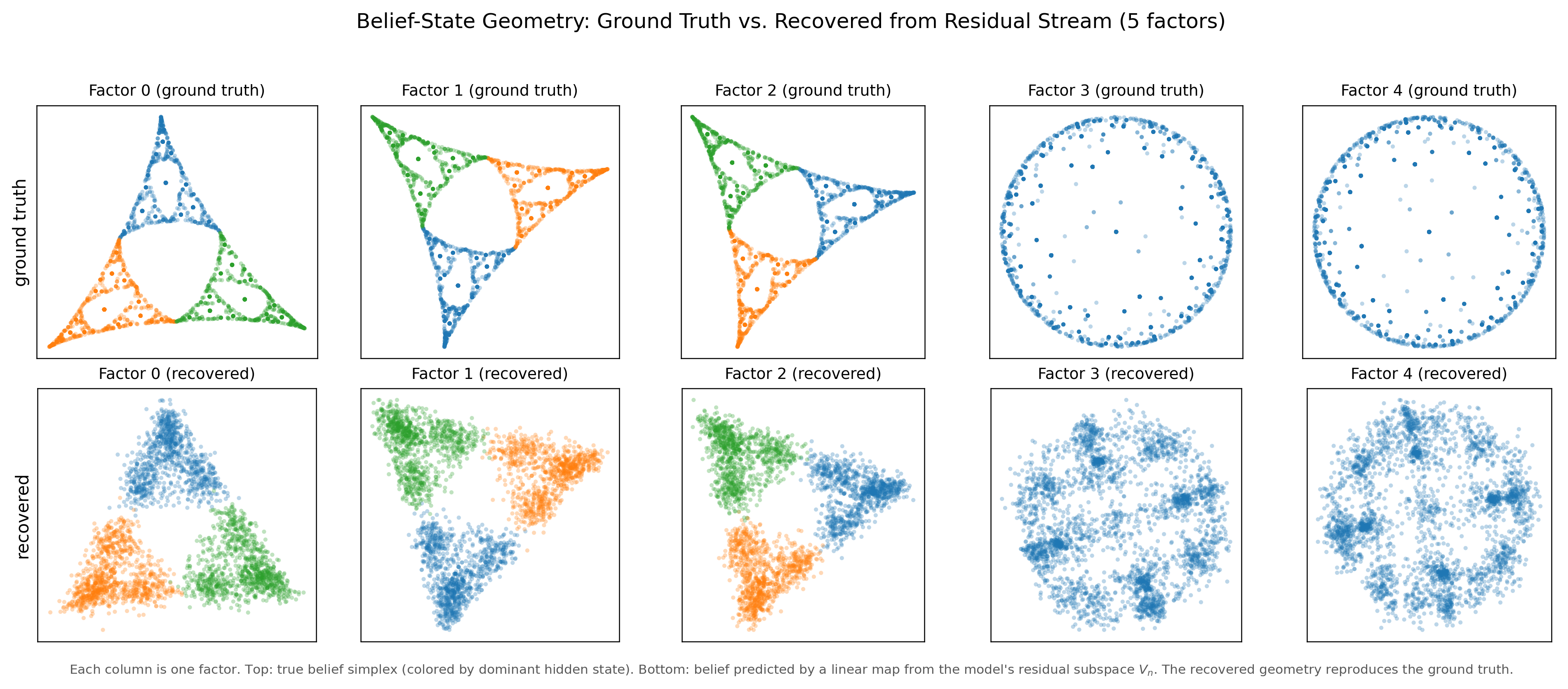 Top: the ground-truth belief triangle per vendor
Bottom: the belief recovered by a linear read-out

[1] The ball is the Bloch ball physicists use to draw a “qubit”; the sphere is just its surface (pure states) and the interior is mixed states.
[2] That is, three mood-odds for a mess3 vendor and three Bloch coordinates for a Bloch-Walk vendor (because even though it has four fruits, the size of its belief is 3).
[3] Later, I ran my own experiment where I widened the stream to $d_{\text{model}} = 480$ and it still factored!